Preparing Experiment Plan files for SHARP.
Good communication is the key to successful shifts on SHARP. It can be the difference between 10 points measured in a shift or 60.
The key to successful experiments on SHARP is good planning and communication. This video describes the most important aspects of experiment planning.
Minimum Required Information
First, we need four primary pieces of information from you.
- NAME: The Mask Serial Number or Name. (IMO314159, Cannonball2, SQ9876, J42PhaseMonster2, etc.) When you ship a mask to us, please send tracking updates to us (when possible), with the mask name, for complete clarity. Sometimes masks have both numbers and names: GORILLA5, JM3712NA. Please tell us both because sometimes only one is written on the box.
- DIRECTION: Please tell us the mask-loading orientation (+y direction). Pictures, drawings, and GDS screen captures of human-readable features, backside bevel locations, etc. all help a lot.
- FIDUCIALS: Three or more fiducial locations. The farther apart the better. These should be features that are relatively EASY TO FIND. Large-pattern corners, fiducial crosses, etc. work best. Finding isolated or otherwise small features can cost time. Features larger than 500 μm are preferred.
- COORDINATES: An Excel or similar file with the measurement coordinates (1) referenced to the center, (2) in mm, if possible.
Creating a File with Graphical Instructions
In addition to the coordinates, it helps to have GDS screen captures, and/or SEMs of the features with clear visual instructions about what we will be measuring, including different length scales that assist us with navigation. In many cases, the fiducial coordinates will bring us to within a few μm of the goals, but if there are any uncertainties (from multiple close-together defects, “perfect” repairs, etc.) having some knowledge about the pattern and labels around the measurement points can save a lot of time.
Many patterns have 3, 4 or 5 nested pattern layers with very similar features. For example, a 10ls10, 2-mm grid of 10×5, 100×200-μm patterns, each with a 2×6 layout of 10-μm-square line regions, containing a 3×3 grid of defects spaced 3 μm apart. Please tell us how to identify and describe the points we are measuring.
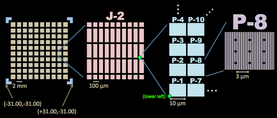
An example of the kind of zoom-in information that can be very helpful in navigating repeated patterns.
Creating an Experiment Plan Spreadsheet
Beyond the minimum essential information and the graphical plan, SHARP users can help us by creating an experiment plan file. Here we describe how to do that. A sample file is shown here, and a downloadable template is available at the link below it.
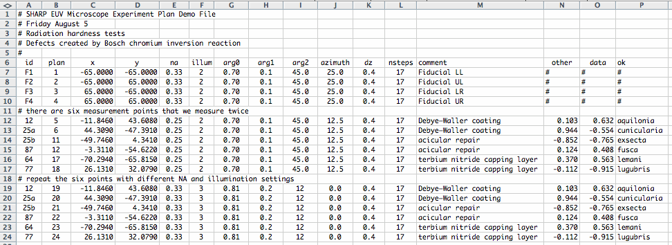
SHARP’s experiment plans are encoded in an Excel-readable CSV format, like this example here.
Excel Template
Download an Excel template here: SHARP_Experiment_Plan_Demo2.xls
General
- # Comments: The pound sign, as the first character on a line, denotes that the line is a comment.
- Headings: Must be lowercase.
- Gaps: There shouldn’t be any gaps in the data. Use a 0 or # to fill in an unused field.
- Commas: Please do not use any commas “,” in the fields. That confuses the CSV format. For comments, commas are OK.
Field Descriptions
- id: Measurement xy location identifier. Alpha-numeric id names can come from other inspection tools, or they be user-defined in any way.
- plan: Sequential and unique numbering of experimental measurements. When the same id (xy) point is measured multiple times, the plan value is different each time.
- x, y: These should be center-based, in mm. We frequently take the μm values given by the users and put those in a column to the right. Then use the spreadsheet to divide by 1000.
- na: This is the 4xNA value. Available values at this time are {0.25, 0.33, 0.35, 0.42, 0.50, and 0.625}.
- illum: The chart below specifies the available illumination settings, which are defined by one pattern value {1-15}, and three arguments, {arg0, arg1, arg2}.
- arg0, arg1, arg2: Partial coherence σ values are scaled from [0,1] on the specified NA, with 1 being the edge of the pupil. Angles are in degrees, CCW from the x-axis. For Disk and Annular pupil fills, Arg2 should be set to 12. This is how many nested circles are drawn for each pattern.
- azimuth: This is the zoneplate azimuth for cross-smile experiments. Available azimuths are {-25°, -12.5°, 0°, 12.5°, 25°}.
- dz: The through-focus step size in μm, in mask units. For 4x and 5x wafers equivalent values, divide by 16 and 25, respectively. For SHARP a typical value is 0.6 for 0.25 NA, and 0.4 for higher NAs.
- nsteps: The number of through-focus steps in the series. Should be an odd number. We try to ensure that best focus is close to the center of the series. We recommend at least 15 steps, although 17 is better when the step size is 0.4 μm.
- additional fields: Users can add arbitrary additional fields to the file; they will be ignored by the SHARP control software. Please make sure there are no empty fields or commas.
SHARP Pupil Fill Patterns
The table below shows the definitions of the illum field {1-15} and its 3 arguments {arg0, arg1, arg2}. Note that all pupil-fill measurements are made on a unit-disk with 1 as the pupil NA’s outer radius. All angles are in degrees CCW from the x-axis.
SHARP is capable of generating arbitrary pixellated pupil fill patterns, such as those being developed for source-mask optimization (SMO). Both binary and grayscale intensity levels are possible. To request and specify such patterns, please work with Kenneth Goldberg and the SHARP team.
1. Monopole
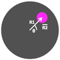
- arg0: R1
- arg1: R2
- arg2: θ
2. Dipole
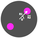
- arg0: R1
- arg1: R2
- arg2: θ
4. Quadrupole
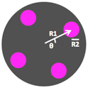
- arg0: R1
- arg1: R2
- arg2: θ
3. Disk
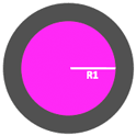
- arg0: R1
- arg1: 0
- arg2: 12
3. Annular
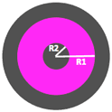
- arg0: R1
- arg1: R2
- arg2: 12
5. Quasar 0°
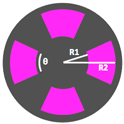
- arg0: R1
- arg1: R2
- arg2: θ
6. Quasar 45°
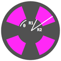
- arg0: R1
- arg1: R2
- arg2: θ
12. Crosspole 0°
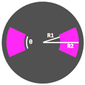
- arg0: R1
- arg1: R2
- arg2: θ
13. Crosspole 45°
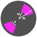
- arg0: R1
- arg1: R2
- arg2: θ
14. Crosspole 90°
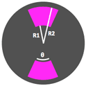
- arg0: R1
- arg1: R2
- arg2: θ
15. Crosspole 135°
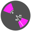
- arg0: R1
- arg1: R2
- arg2: θ
