
Information about the data generated by the SHARP EUV Microscope
This page describes the formatting and structure of image data collected on the SHARP microscope.
File-naming convention
The filenames are defined according to the following pattern.
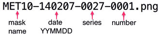
Format
SHARP images are 16-bit grayscale PNG files (0–65535 unsigned integer), stored with lossless compression. A typical raw image file can be downloaded here: MET10-140207-0027-0001.png [5.4 MB] (This 16-bit file may not render properly in your browser.)
Image Size [pixels]
Images are 2048 x 2048 pixels, representing the full CCD Camera. Typical images span approximately 30 μm with approximately 15 nm per pixel, in mask units. (Lenses with 4xNA values about 0.35 have higher magnification ratios.)
File Size [MB]
Average file size is 5.7 MB. A busy 8-hour shift can produce close to 7 GB of image data.
Orientation
Beginning February 2014, the image orientation has been y-flipped relative to prior data. Now, most image-reading programs will show the image properly with +y toward the top, and +x to the right, relative to the mask. Data recorded before February 2014 has a y-flip as it comes directly from the CCD camera.
Metadata 1
Beginning February 2014, human-readable metadata is stamped in the lower right shadow region of the image. The metadata contains basic image and illumination settings, comments, and a length scale-bar which should be interpreted as being approximate. An example image is shown below, with a detail of the metadata stamp region.

An EUV (actinic) mask image from the SHARP microscope. [Click to enlarge.]

Enlargement of the metadata region
Metadata 2
Beginning February 2014, machine-readable metadata is inscribed along the bottom 1–3 rows of the image in ASCII format. This includes all of the metadata collected by SHARP with each recorded image. The data is easily read and parsed, as text strings. The format details are described in this memo: SHARP image file metadata stamping and encoding. [PDF] As described in the memo, images stamped with metadata start with a sequence of five 1s in the lower-left [0,0] pixel, moving in the +x direction. Note. The ASCII data is converted to integer values from 0 to 255. Therefore, it will appear darker than the typical CCD values in the shadow region, which can be close to 500 counts due to the hardware offset value.
Background Level
The circular shadow of the MC mirror is visible near the bottom part of the SHARP images. The shadow region, to the left of the metadata, provides a convenient means to assess the background level of the CCD camera, which comes from (exposure-time dependent) dark current and an intentional offset imposed by the CCD hardware. The image detail below is overexposed to show the shadow region.

We recommend extracting the average CCD pixel intensity within the box defined by
x ∈ [8:255] and y ∈ [16:63]
counting from a zero-index. Here, we avoid a bright pixel column that can occur on the left edge (column 0), and we stay above the machine-readable metadata which is along the bottom few rows of the image in y.
Please note that background subtraction is essential for all accurate measuremens with SHARP. After mathematically subtracting the background level, the intensity levels in the image will be proportional to the photons collected at each position. Without background subtraction, all measurements (contrast, NILS, CD, etc. cannot be accurate.)
Image Sweetspot
Although SHARP images show a region that spans over 30 μm width, the zoneplate lenses have a relatively small sweet spot where the aberrations are minimized. The position of the sweet spot is determined by the operator of SHARP during the data collection (based on qualitative feedback), and we try to maintain a consistent position throughout a given shift. The metadata value, image_sweetspot contains the pixel location of the sweet spot, represented as “(x;y)”. We generally say that the sweet spot area covers up to 3 μm radius from the center of the sweet spot, but this value is NA dependent. Small NAs have a large sweet spot, and higher NAs have a smaller sweet spot. All quantitative image analysis should be conducted within the sweet spot region; data outside of this region is not reliable due to increasing aberrations, dominated by astigmatism.
Focal plane tilt
The off-axis geometry and single-lens imaging in SHARP gives the images a vertical focus gradient, or focal-plane tilt. (The tilt increases with increasing central ray angles.) Users will observe that points in the image that are separated in the y direction will come into focus at different z positions. In general, analysis of vertical line features across 2 μm distances will not be significantly affected by the focal plane tilt.
Illumination uniformity
In SHARP we make a trade-off between flux density and uniformity in order to keep a reasonable exposure time. Therefore, we concentrate the available light into a region that is approximately 10-μm wide, or slightly smaller. Our goal is to produce uniformity levels better than 2% across the sweet spot where analysis will be performed. Users should not expect flat illumintion across larger regions than this for conventional settings. If your experiment requires uniformity over larger areas, please let us know specifically, in advance of your shift. There will be a necessary increase in the exposure time to reach sufficient SNR in the sweet spot.
Image Rotation
In SHARP we observe that there is a small rotation of the mask on the mask holder, relative to the CCD camera. Between June 2013 and May 2014, this rotation was 1 to 1.5°. Accurate measurement of pattern properties requires the removal of this rotation.
Vertical Motion Through Focus
The off-axis illumination in SHARP produces an apparent (non-telecentric) motion of the image through focus, mostly in the vertical direction. To a great extent, the observed motion tracks the central ray angle of the illumination (typically 6°), and does not have a horizontal component. More exotic illumination settings, or small errors in the central ray angle, can influence the observed motion in the image stack. In addition, small, lateral errors in the stage motion can produce unpredictable image shifts on the scale of a pixel or two, away from the expected positions. In cases where the through-focus measurements require stationary alignment on mask features, we recommend applying a fine lateral image shifting based on comparisons of sequential images in the stack. Sub-pixel interpolation, based on Fourier-domain autocorrelation, has proven successful in many common cases. To predict the expected image motion through focus, use the central ray angle (often 6°) and the mask-side focal step size (commonly 250–500 nm), and the effective pixel size of the CCD (close to 15 nm when standard 0.33-4xNA zoneplates are used).
CSV Imagelog File
Metadata from a single day is preserved in an Excel-readable, CSV (comma-separated value) text file. The file name begins with “imagelog,” contains the organization/company name, and the date (formatted as YYYY-MM-DD), like this imagelog_lbnl_2014-02-07.csv. Comment lines begin with #.

We are now recording additional image metadata that had not been fully implemented until April 2014. These include the important parameter image_sweetspot. This is an xy image pixel location where the SHARP operator has targeted the data collection. The format is (x;y) = “(1234;976)” as a string. (Note: Rows and columns are counted from zero.)
"detail" Folder (thumbnail images)
Beginning April 4, 2014, SHARP software now creates image-detail thumbnails, one per series, using the central image in each through-focus series. The files are small, intensity-scaled JPEGs, centered on the operator-defined sweet-spot, and covering a square area with 1/4 of the full camera width. For NA values ≤ 0.35, this is about 7.68 μm. The thumbnails are stored with the original data, in a subfolder called "detail". Please note that these files are not intended for quantitative analysis. They only provide a quick view of the sweet spot region.